

Introduction

Cleaning. Sometimes challenging. Even with the right tools. Image: Bath Time by archer10. Some rights reserved CC-A-SA 2.0.
What is this recipe and what do you get out of it?
Cleaning data is an essential step in increasing the quality of data. This Data Wrangling Handbook recipe looks at six common ways that a dataset is ‘dirty’ and walks through time-saving ways you can use a spreadsheet to fix them and ‘clean’ the dataset.
The recipe is very detailed, because data cleaning is all about attention to detail. Some of it is easy – and you’ll wonder why we included it! But some of it is hard – particularly the later sections on structural problems and inconsistencies. But by the end of it you will have used a set of spreadsheet features and functions in combination with each other to do something useful.
It will help data cleaning become less tedious by showing you how to use the software to do thing you’d otherwise do ‘manually’, with the accompanying risks of missing some errors, and introducing new ones. The techniques we introduce also scale to a certain point. The sample dataset we use has 400 or so rows of data, which is just big enough to be a headache to clean up by going row by row, fixing problems by hand. These techniques will work where you have a lot more data.
It is aimed at people who are familiar with spreadsheets, and requires no knowledge of programming. It uses a range of features and functions of the spreadsheet. The spreadsheet features we will use include:
- Autofilter – quickly find out what’s in a column of data, and show which bits you want
- Conditional formatting – highlight cells of data based on criteria you specify
- Data Validation – choose what values are allowed in a cell
- Defined data ranges – create lists of data that can be used to make comparisons
- Find and Replace – look for one thing, and replace it with another
- Paste Special – remove unwanted formatting
- Pivot tables – summarise your data and see it in completely new ways
- Regular Expressions – clever way of searching for data
- Text-to-Columns – split up cells of data that have more than one entry in them
The recipe also makes use of forumulae that use some different spreadsheet functions, including CLEAN, CONCATENATE, COUNTA, IFBLANK, LEFT, SEARCH, SUBSTITUTE, and TRIM. You may not have known these existed, but they can speed up a lot of the most difficult and time-consuming parts of removing errors from a dataset.
The recipe is a complete process, showing every step. It can be a useful learning aid, guide or reference point for you in managing your own datasets. Finally, this recipe is the ‘textbook’ for a School of Data Course called A Gentle Introduction to Data Cleaning which is a more accessible and engaging way into this quite dry topic.
Get set up: data and tools you will need to follow this recipe
Software tools used in the recipe
The spreadsheet software we have used throughout this recipe is part of Libre Office 3, which is free, open source software that works on Windows, Mac and Linux operating systems. Libre Office 3 can be downloaded and installed from the Document Foundation website. For help getting set up have a read of the free installation guides (they’re quite good).
Most of this recipe can be also be used in recent versions of Microsoft Excel and Google Spreadsheet. The screenshots will look different and the steps may not be quite the same though. To help complete some tasks, we will also occasionally dip into a word processor and text editor like Notepad. These will probably already be installed on your computer.
The ‘dirty’ data – what we’re starting with
We will be working with a spreadsheet of data about sales of vast amounts of agricultural land in less developed countries. The data was researched by a non-governmental organisation called GRAIN, which works to support small farmers and social movements in their struggles for community-controlled and biodiversity-based food systems.
We have placed a spreadsheet with the original dataset on the Data Hub, an online library for data. To follow this recipe, you will need to download a copy of this onto your computer.
The ‘clean’ data – the end result
By the end of this recipe, the data will be substantially cleaned up. We’ve put a copy of the original data along with the final, cleaned GRAIN data online too.
Problem 1: Showing the data plainly
What’s the problem?
Spreadsheets are visual tools that give you control over the way text and numbers are displayed: this is called formatting. It can be helpful, and help display the data in ways that make it easier to use and understand. It can also be unhelpful make data more difficult to see.
Before moving forward, look at how the GRAIN data is currently displayed:
- The text is very small. This is maybe to try and fit all the data on the screen so you don’t have to scroll right to see it.
- There is some colouring in there. Why? What does it mean? Does it signify something important about the data?
- Can you find any hidden rows or columns? Look for discontinuities in the column lettering and row numbering.
What’s the solution?
Use the cell formatting features
To display the data in a plain and compact way, removing any choices that the original publisher of the spreadsheet made, you can do the following:
- Select the complete dataset (Linux/Windows shortcut: Ctrl+A).
- With the data now selected, right click on top of any row label (eg. 1, 2, 3 etc) to bring up the secondary menu. Choose “Show”. This will make sure any rows that are hidden are revealed. Repeat the same steps for the columns.
- With all the data selected, right click anywhere to show the secondary menu. Select “Clear Direct Formatting” to remove cell colouring and make the text size uniform.
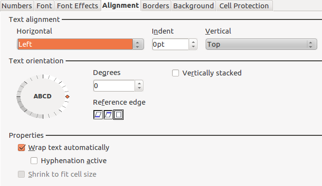
Right click again, and go to “Format Cells”. Select the ‘Alignment’ tab and choose the following options to place the text sensibly in the cells:
- With all the data still selected, right click on any row label again and choose “Optimal Row Height”, and select ‘Okay’. This will resize the rows to remove extra vertical space, which results in more data being displayed in-screen.
- To resize the columns, place the mouse cursor in the line between columns. Left click and hold, and drag the line until you’re happy with the column width.
Problem 2: Whitespace and new lines – data that shouldn’t be there
What’s the problem?
Apply autofilter to the GRAIN data in the worksheet (Data →Filter → Auto-Filter). Bring up the select list for “Status of Deal” by choosing the downwards-pointing triangle that has appeared in the column label, as below:
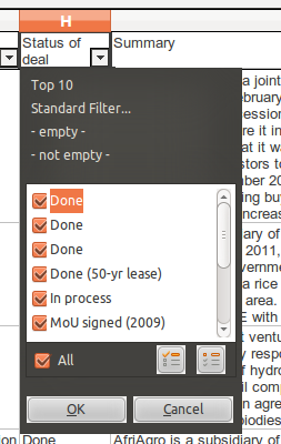
Why are there three entries for “Done”? Look at the selection list for other columns? Can you see where there are other duplicate entries?
The reason for the duplicate entries is that there are extra characters alongside the data that are not displayed – so you can’t easily see them. These are likely to be either whitespace at the ends of lines (also called ‘trailing spaces’ or new lines that were added accidentally during the data entry. These are very common errors, and their presence can affect eventual analysis of the data, as the spradsheet treats them as different entries. For example, if we are counting deals that are categorised as Done, the spreadsheet will exclude those that are categorised as “Done “ (note the extra space at the end).
Similarly, cells can also have new lines in them, the presence of which is obscured by the layout. For example, find the cell containing the text ‘Libyan Investors’. On a first glance it looks fine, but double click to edit it. There is an extra line beneath the word ‘investor’, as illustrated by the presence of the cursor beneath the text:
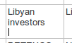
Entries for ‘Libyan investors’ with and without a new line afterwards are treated by the spreadsheet as different data. In turn, this will affect the accuracy of data analysis.
What’s the solution?
There are two easy ways to remove whitespace and new lines from a worksheet. Both are equally as effective.
Use the Find and Replace feature
Both whitespace and new lines can be “seen” by the spreadsheet.
- Open the find/replace tool (Shortcut: Ctrl-H).
- Select “More Options” and check “Regular expressions”. This feature enables the spreadsheet to search for patterns, and not just specific characters.
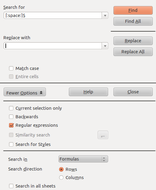
In the input area for Find type [:space:]$ and click “Find”. This is a regular expression that searches only for spaces that are at the end of the text in a cell (which is what the $ denotes). It should look like this:
- Running this search will show you the cells in this worksheet that have one or more trailing whitespaces.
- To remove the trailing whitespace that have been found, click “Find All”. Make sure the input area for ‘Replace with’ is empty. Then click on “Replace All”. Perform this operation until the spreadsheet tells you, “The search key was not found”.
- To remove the new lines, repeat steps (a) to (e) with n in the Findbox. Remember to keep regular expressions enabled, or this won’t work.
- Run the auto-filter again to see how the data has changed.
Use the TRIM and CLEAN functions
Trailing whitespace and new lines are common enough problems in spreadsheets that there are two specialised functions – clean and trim – that can be used to remove them. This is a little more detailed, so follow the steps carefully:
- In your spreadsheet, the GRAIN dataset should be in ‘Sheet1’. Create a new worksheet for your spreadsheet, called Sheet2.
- In cell A1 of the new worksheet you have just created enter the following formula: =CLEAN(TRIM(Sheet1.A1)) and press enter. This will take the content of cell A1 from Sheet1, which is your original data, and reproduce it in Sheet2 without any invisible character, new lines or trailing whitespace.
- Find out the full data range of Sheet1: It will be A1 to I417. In Sheet2, select cell A1 and then copy it (Shortcut: Ctrl+C). In the same sheet select the range A1 to I417 and paste the formula into it (Shortcut: Ctrl+V). The complete dataset from Sheet1 will be reproduced in Sheet2, without any the problematic invisible characters.
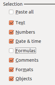
- To work further on this data, you will have to now remove the formulas you used to clean it. This can be done with the Paste Special operation. In Sheet2, select the complete dataset and copy it. Put the cursor in Cell A1, and then go to Edit → Paste Special. This enables you to choose what attributes of the cell you want to paste: we want to paste everything except the formulas, which is done by checking the appropriate boxes, as below, and then clicking Okay:
-
Double click on any cell, and you will see that it just contains data, not a formula. If you like, run through the steps outlined in Problem 1 to make the text ‘wrap’ in cells, and adjust the column widths.
Problem 3: Blank cells – missing data that should be there
What’s the problem?

In many spreadsheets you come across there will be empty (“blank”) cells. They may have been left blank intentionally, or in error. Either way, they are missing data, and it’s useful to be able to find, quantify, display and correct them if needed.
What’s the solution?
Use the COUNTBLANK function
This will enable you to show the number of blank cells, which helps you figure out the size of the potential problem:
- Scroll to the end of the dataset. In a row beneath the data, enter the following formula: =COUNTBLANK(A1:A417) and press enter. This will count the number of blank cells in column A so far as row 417, the last entry in the GRAIN dataset.
- In the same row copy the formula you just created across rows B to I. This will show you a count of the blank entries in the other columns.
- You can see that by far the most blank cells are in column G, ‘Projected Investment’.
Use the ISBLANK function with the Conditional Formatting feature
Blank cells can also be highlighted using conditional formatting and the ISBLANK function, changing the background colour of blank cells, so you can see where they are:
- Select the dataset (cells A1 to I417), and open the ‘Conditional Formatting’ menu (Format → Conditional Formatting → Conditional Formatting). This spreadsheet feature allows you to automatically change the formatting (eg. font size, cell style, background colours etc) depending on the criteria you specify.
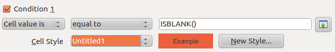
In the conditional formatting window, make the conditions look like the image below. To make the blank cells stand out more clearly, use an existing style or set up a new one by clicking the ‘New Style’ option, which takes you to a window where you can choose font type, size, background colour and so on.
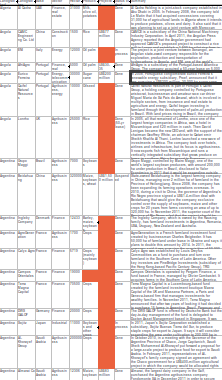
Check what has happened. When the conditional formatting is applied the blank cells will be highlighted in red. Here’s how it looks when zoomed out a bit (View → Zoom, then enter 75% into the ‘Variable’ option):
To remove the conditional formatting: repeat steps (a) to (b) above, but define a clear style (or use the ‘default’) instead. Otherwise select the cell or range of cells and select “Clear Direct Formatting”.
Fill in empty values with the Find and Replace feature
In the GRAIN dataset we do not know whether blank cells signify data that has been deliberately or accidentally left out. You may want to actively specify that the data is missing, rather than leaving a blank cell.
- Select the complete data range (A1 to I417).
- Open the find/replace dialogue (Shortcut: Ctrl-H). If you have already used this earlier, you will need to disable searching with regular expressions, because this causes the search to work differently. Do this by clicking ‘More Options’ and uncheck regular expressions.
- Leave the “Search for” input box empty. Type “Missing” into the replace box (without quote marks). Click on ‘replace all’.
- Every blank cell will now have the value “Missing” recorded in it. You can verify this using the COUNTBLANK function we outlined above.
Filling blank cells isn’t always useful and it’s important to choose the right term to denote a missing value. For example, in the context of ‘Proposed investment’ using the term ‘none’ to signify missing data is confusing. Readers may think this means you know there is no investment, rather than that there is no data.
Problem 4: Fixing numbers that aren’t numbers
What’s the problem?
The GRAIN dataset has a column called Proposed Investment. This records the amount of cash paid for land in US Dollars. However they are recorded as text, not as numbers. This means the spreadsheet can’t use these values to do the mathematical operations required to make totals, averages, or sort the numbers from highest to lowest. Further, the data have not been entered in a consistent form. Here are some examples from the dataset:
- US$77 million
- US$30-35 million
- US$1,500 million
- US$ 2 billion
- US$57,600 (US$0.80/ha)
So the problem is twofold: there is no consistent unit, and there are data other than the currency in the cell. Ideally, what we would have are data like this:
What’s the solution?
We can solve this with a combination of automation and old-fashioned hand correction of data. A part solution using a combination of formulas
- Choose a consistent unit: US$ millions.
- Create a new column H called “Projected Investment (US$ millions) to the immediate right of the current column G, Projected Investment. We will use column H as a working column to display the outcomes of our calculations.
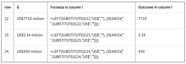
- Go to Cell H2, and enter the following formula: =LEFT(SUBSTITUTE(G2,”US$”,””), SEARCH(” ”,SUBSTITUTE(G2,”US$”,””))) Then copy it (Shortcut: Ctrl-C).
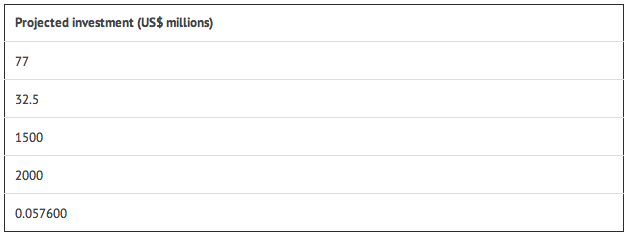
Select the range H1 to H417 using the mouse, and paste the formula into that range. You will see that if there is any data in Column G, a new value will be displayed in column H, as below:
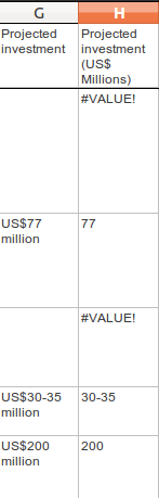
Where there is no data, a warning sign like #VALUE! will be shown.
- This formula works using three functions joined together: LEFT, SUBSTITUTE and SEARCH.
That’s some crazy stuff, dude! Explain yourself.
It’s complex but a good exercise in thinking about what data is, and how spreadsheets can process text quite effectively by combining different functions into formulas.
Let’s start with the simplest and most common sort of case from the GRAIN database:
US$77 million
We want to turn this into a number that the spreadsheet can work with:
US$77,000,000
There are two things that we can immediately do: specify the currency as an attribute of all numbers in the column “Projected investment” so we know that all numbers in this column are US$. This removes the need to put the text “US$” in each cell:
77,000,000
As nearly all the entries are over 1 million in size, it’s sensible to specify that all numbers in the column “Projected investment” are in millions. This removes the need to include the trailing zeros – the 000,000 – in the cells. This leaves us with:
77
So, the actual task the formula needs to do is to change “US$77 million” to “77”. We want to remove everything but the number 77, with as little potential for error as possible and in a way that can be applied to as many of the other data in the ‘Projected Investment’ column as possible.
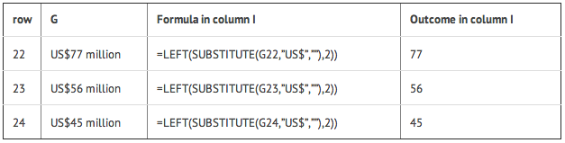
This is where the LEFT function comes in. Look at the value we want to change: US$77 million. Count the characters, including the spaces: there are 13 in total. The LEFT function reads the value, and displays only characters to the left of and including the character number you give it. Here’s how it works on the value “US$77 Million”:
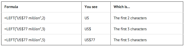
In the above examples we included in the formula the actual text that we wanted to analyse using LEFT. We can specify which cell we want to analyse (this is called cell referencing). For example, in the spreadsheet we might have:
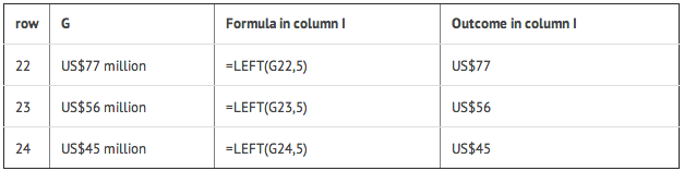
Building the formula this way enables it to be copied down a column, as the cell numbers will update automatically as the position of the formula changes. We can further improve the formula and remove some of the text that we ask LEFT to analyse. This is where the SUBSTITUTE function is useful. Here’s how it works, then we’ll apply it in combination with the LEFT function:
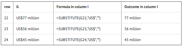
The SUBSTITUTE function takes the content of a cell (eg. G22, which has the text US$77 million), looks in it for the specific text you tell it to (in this case “US$”), then substitutes it with what you tell it to (in this case, for “”, which is nothing at all) and prints the result (77 million).
We can combine SUBSTITUTE with LEFT. So, in the below, LEFT does its work on text that has already had characters removed through the SUBSTITUTE function:
So, we have the numbers we need now but there is a problem. Not all the original numbers recorded in ‘Projected Investment’ are 2 digits long. Here’s what happens if we run this formula on a more varied set of data in the G column:
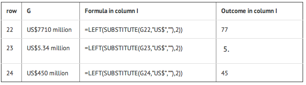
Uh oh! You can clearly see there are mistakes in the outcome column. This is because we have told LEFT to show only 2 characters each time (remember we have removed the “US$” using SUBSTITUTE, so LEFT doesn’t count those). However, to show the correct figure for “US$7710 million” in row 22, LEFT would have to count 4 characters. So how can we give LEFT the correct number of characters?
Look at the values again. They have something else in common: yes, they have a space separating the number from the text “millions”. Its position will vary each time but we can find it tell the LEFT function to show it where the number ends in each case. The SEARCH function can be used to do this. It works by looking through data you give it for a character you specify, and then tells you the position of that character:
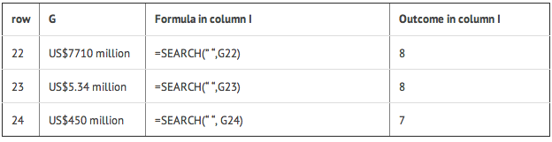
So, in row 22, we are looking for a space (“ “) in the text in cell G22 (US$7710 million). Count from the left, that space is in position number 8. We can give this number 8 to the LEFT function:
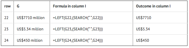
Note that these outcomes also include the space after the number. Let’s add the SUBSTITUTE function back into the formula: Wherever there is a cell reference (eg. G22) we can put a SUBSTITUTE function removing the text US$:
That explanation help?
Refine the solution to remove the errors
Throughout this example, you can see how a useful formula can be built up to help solve the problems we outlined at the beginning. However, taking this approach leaves us with loose ends, for example:
- Where there is no data in column G, this formula will not know what to do, and will return a #VALUE! error, which makes it more difficult to use the new data in other calculations.
- If the value is US$22 billion rather than $22 million the formula will still return 22. The correct value in a column of data in US$ millions should be 2200.
- If the value is US$30-35 million, the formula will return the range 30-35, rather than a single value.
- Where a value is below a million, and has some additional explanation, such as in “US$57,600 (US$0.80/ha)”, the formula will return 57,600. In a column demoting US$ millions this would be a huge amount.
We use formulas to automate the process of cleaning data to the greatest extent possible but there will always be exceptions. The key is to know where the exceptions are and decide whether it is worth continuing to try and accommodate them with a formula, or whether to just correct them by hand. How do we do this? We can use a feature of the spreadsheet called a Pivot Table. This will help us find the troublemakers, how many of them there are, and whether we should continue to fix with formulas by hand.
Use a Pivot Table to find errors and Autofilter to help fix them
- At this point your, dataset should have the original Projected Investment data in column G, and the cleaned data in column H, which we named Projected Investment (US$ MIllions).
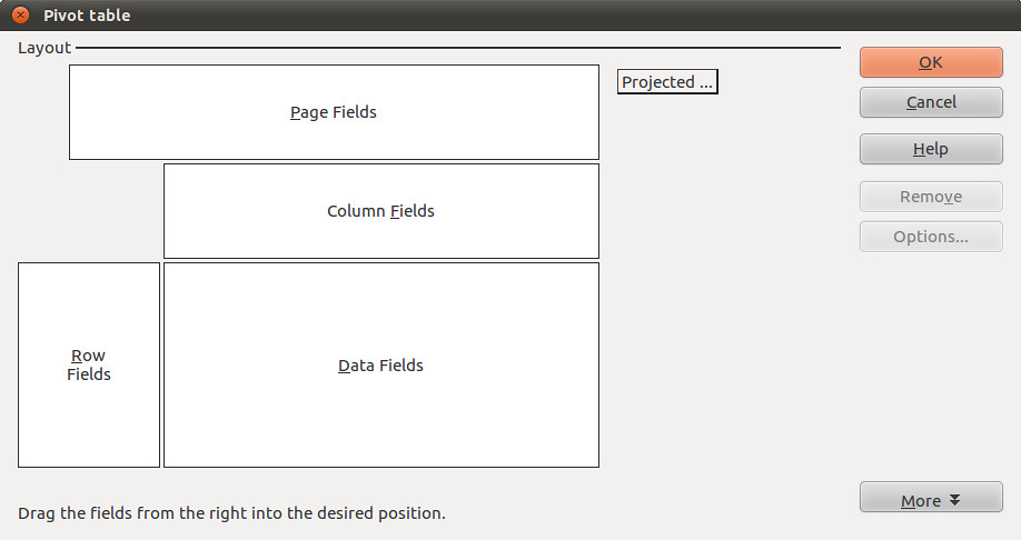
- Select column G. Go to Data → Pivot Table → Create New. In the window that appears, checked “Current Selection” and click on OK. A strange new window called Pivot Table will appear, which looks like the image below:
- We can use this to find a list of the unique values in column G (Projected Investment), which will help us identify trouble-causing entries. Select the little grey rectangle near the top centre labelled “Projected…” and drag it to the white area called Row Fields. Select it again and drag it to Data fields too. You should see this:
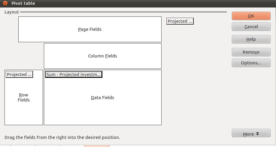
Notice that in the Data Fields, the little grey rectangle is now labelled “Sum – Projected Investments…”. We want to change this to “Count – Projected Investment … ”, so it shows us how many times each of the different values occurs in the dataset. To do this, double click on it. This window will appear:
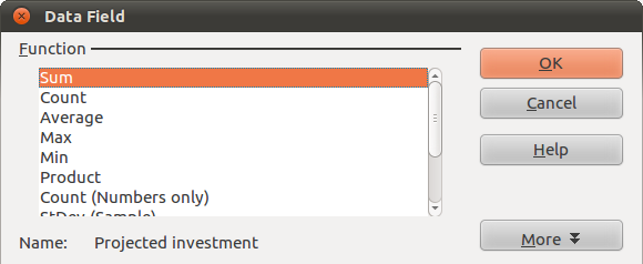
Select Count. Then click Okay in the pivot table window. A new worksheet will appear, containing a list of unique values from column G, along with the number of times each occurs.
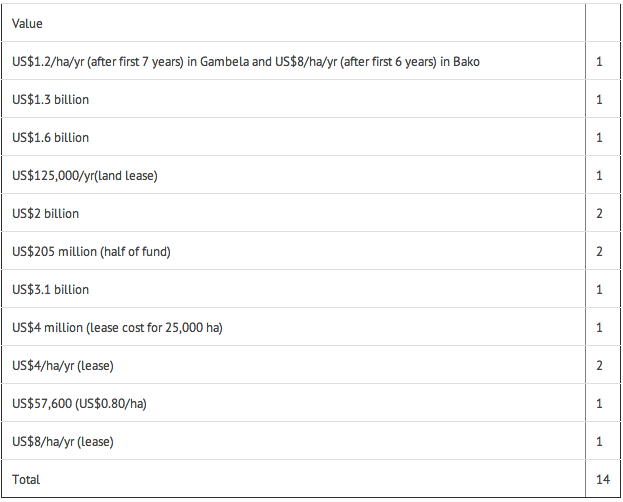
- This view of the data enables us to quickly scan down the list and see the problems. The count lets us know how much work it is likely to be to fix them. So, with a quick bit of analysis of this pivot table, we can see that of a total 416 rows of data in the GRAIN dataset only 106 values (that is 416 minus the 310 where data are not present) are recorded in the column for Projected investment. Of these 106, only 14 are NOT uniform like “US$34 million” or “US$1,876 million”. Here are the offending entries, which we’ve pulled out into a table:
We can fix these in about 5 minutes simply by identifying them in the original data, and changing them by hand so our formula can then process it. Head back to the worksheet you have your clean data in. A quick way to highlight these entries is to use the autofilter selection list that we used above.
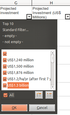
Go through the list and make sure that only the exceptions we have identified are selected. Then click OK. This will change what the spreadsheet shows: only those rows that have in column G the data you’ve selected will be shown. You can now go through them one-by-one, changing the data in column G so the formula we made can work on it. You will see the results in Column H, which will update automatically. For example:
US$30-35 mil → hand correct into an average: US$32.5 million → Formula returns 32.5
US$2 billion → hand correct in US$2,000 million → Formula returns 2,000
…and so on.
Tip: as you are updating original data, you may wish to keep a note of what you changed. Either create a column called “Notes”, and record the data there. Or, duplicate column G and name this new column “Projected Investment (un-altered)”. Or, where appropriate update the column called “Summary” with the data, which is the approach we have taken.
There are a few final steps to take to make the numbers in column H usable. Currently, our data in column G is a calculated value, not a number: in spreadsheet language, this means we can’t add them up yet! We need to replace the formula with its result. This is easily done with the Paste Special feature we noted above.
- Select the whole of column H (or just H1 to H417 if you prefer).
- Copy it (Shortcut: Ctrl-C). Put the cursor at the top of column H, selecting Cell H1. Go to Edit → Paste Special. A window will appear, like this:
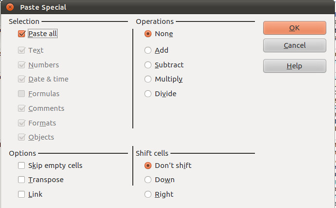
- We can choose what aspects of the selected data are pasted by checking and unchecking them. Make it so it looks like this, then select OK:
- Edit one of the cells in column H. You should see that the formula is gone, and there is only a number. Sometimes, after a Paste Special operation, when you edit a cell you may also see an apostrophe has been inserted into the number. This is an infamous bug. You can remove the apostrophes by selecting the column, going to Data → Text to Columns. Just select OK, and the problem will be fixed.
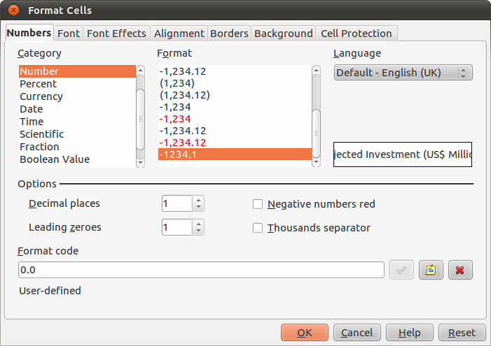
- Finally, format your column of numbers correctly. Select the column (or range H1:H417), right click on the selected area to bring up the secondary menu. Choose “Format Cells”. In Numbers, select the category ‘Numbers’, and choose -1234, and then change the value for Decimal places to read “1”. Then click OK.
- Now your numbers are ready to use.
Problem 5: Structural problems – data in inconvenient places
What’s the problem?
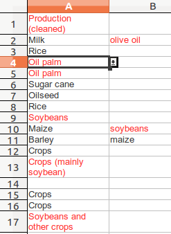
Look closely at column F of your increasingly clean GRAIN dataset. This contains details about the intended use to which sold land will be put. Here are the first 10 entries (if your sheet is sorted alphabetically by ‘Landgrabbed’):
- Milk, olive oil, potatoes
- Rice
- Oil palm
- Oil palm
- Sugar cane
- Oilseed
- Rice
- Soybeans
- Maize, soybeans, wheat
- Barley, maize, soybeans, sunflower, wheat
In some cells there are single values, like just Oil palm. In others, the picture of how land is used is more complicated and there are more values. At a simple level, this data means we can do some basic analysis. Try this:
- Let’s try and find all the land deals where Alfalfa was to be produced. Select the complete dataset. Go to Data → Filter → Autofilter. You’ll see the little triangles appear on the column headings, like so:
- Select the little triangle, and a selection list will appear, which contains a list of all the values column F, listed alphabetically and without duplicates. Choosing from this list will change what data is shown in the spreadsheet:
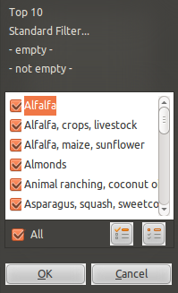
- In this list, untick Alfalfa. If you clicked “OK” now, the spreadsheet would show all rows of data that have everything but Alfalfa in column F. We can reverse this by unchecking Alfalfa and selecting the reverse button (at the bottom right of the window above you see two pictoral buttons, choose the left one). This reverses things, and shows only the unselected values. Click “OK”, and you will see only rows of data where the single word Alfalfa is present in column F. There are only two.
- There are clearly other records where Alfalfa is recorded in Production. Repeat the above steps but include the items on the list that say “Alfalfa,crops,livestock” and “Alfalfa,maize,sunflower”. With this filter there are 2 more rows of data, showing us 4 deals where Alfalfa was grown.
- To remove the filter and again show all your data, go to Data → Filter → Remove Filter.
So we can do some useful basic stuff. But there are problems that will affect the analysis:
- We can’t see the complete range of options very easily.
- We have to rely on the people creating the data to have arranged things alphabetically too; what if someone had recorded Alfalfa at the end of the list? We couldn’t see it.
- Further, we assume they’ve spelled things the same each time, or used the same word for example: “Alfalfa crop” or perhaps another word for it.
- It’s difficult to get a full list of the land uses that you can look for.
What’s the solution?
In a spreadsheet this can be partially overcome using the standard filter, which is more flexible than an autofilter.
Use standard filters for a more flexible search
- Go to Data → Filter → Standard Filter. This opens up a window like the one below. It has a lot more options. Let’s look for deals involving Alfalfa again. Make your standard filter look like this, and select OK:
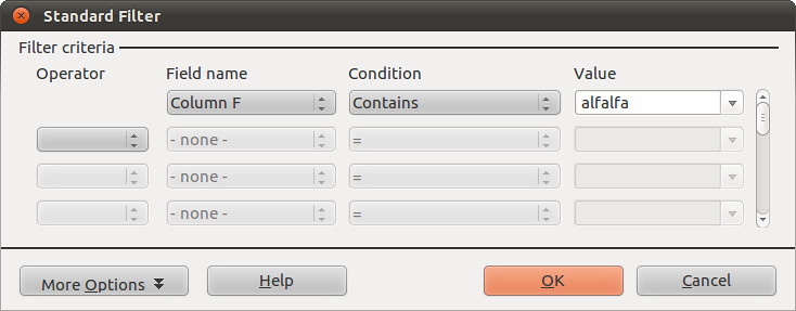
- So, this searches down Column F, where our data about production is stored, for cells where the word “alfalfa” is written anywhere. It doesn’t matter whether other words are there. The spreadsheet will again be filtered to show four rows.
- We can build up more complicated queries. For example, try this one, which will filter the data for deals where the land use was thought to be for rice AND bananas, amongst others:
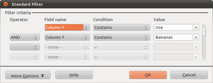
- This returns only two results.
- To remove the filter, go to Data → Filter → Remove.
Why this is only a part solution
Again, it’s sort-of-useful but quite limited for the same reasons as autofilter: mis-spellings, alternative wording, not having a complete list to choose from. At root this is a very difficult problem to solve with a spreadsheet: data on Production is what we call a repeatable field, in that buyers of land can have many equally important uses for the land. This is a different dimension of data: it’s called a one-to-many relationship. There is no easy way to structure data for a spreadsheet to make this data easy to use with any accuracy.
A common mis-step at this point is to start adding columns to allow multiple data to be recorded. This isn’t any better than recording it all in one cell, because of the way spreadsheet filters work. For example:
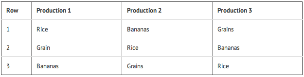
In the example above, all three rows have entries for “Rice”. A spreadsheet filter looks only up and down a column, not left and right to other columns. So to build a filter that accurately returned all three rows, you would need to search all three columns for the term “Rice”. This quickly becomes impractical as you begin wanting to find rows with different combinations of production types.
At this point, altering the structure of the GRAIN data for use in a spreadsheet probably isn’t worth it as there would be little gain. However, in this dataset, around 30% of entries in this column have more than a single entry, and there are nearly a 100 types of production. Having the data is important, as it may allow us to ask and answers questions we wouldn’t otherwise be able to. For example, are there certain land uses that go together? Is there a relationship between the land use, the size of the land transacted, or the amount of investment. Exploiting the data effectively requires a database, not a spreadsheet.
However, there are things we can do to improve our ability to analyse the data, which we will go into in the next section.
Problem 6: from “banabas” to “bananas” – dealing with inconsistencies in data
What’s the problem?
In the GRAIN dataset look again at column F, called ‘Production’. This column contains data about what buyers of land intend to grow on their new acquisitions, such as growing ‘cereal’, ‘soyabeans’ or ‘sugarcane’ and many other types of agricultural activity. As mentioned above, we can use this data to sort and filter the dataset, which helps us see the extent of different kinds of production. However, there are some uncertainties that make the data in the ‘Production’ column far less useful than it could be:
- We don’t know everything we could be looking for in the dataset. This is because there isn’t a single list of categories of production (called a ‘controlled vocabulary’’). There are in fact well over 100 distinct categories. How do we get them into a single big list?
- We can’t be confident that the people creating the data have been consistent in how they entered the data. So if we look for “oil seed”, you’ll also find “oilseed” and “oil seeds”. This difference is important because a spreadsheet treats these these as completely different things.
We can address these obstacles to our understanding of the data. What we are going to do is create a new, more accurate and consistent controlled vocabulary for this dataset and apply it to the data. Here’s how.
What’s the solution?
The process of solving this problem has four steps, which we’ll cover in detail:
- Get all the categories that appear in the data
- Make one big list from the almighty mess
- Remove duplicates and correct categories that are nearly the same
- Edit the data to fit the more accurate list of categories
Get all the categories that appear in the data
As we discussed above in the section on structural problems, different pieces of data about production are held in a single cell. Each item is separated by commas. We can use a feature called “Text to Columns” to separate out each of the items into individual cells.
- Create a new empty worksheet and name it “Text-to-columns” (or something memorable so you know what’s in it). We will use this worksheet as a ‘scratch pad’ to work on this particular problem.
- In the GRAIN dataset that you have been working on, select Column F containing the data about production. Copy it (Shortcut: Ctrl-C) and then go to your new “Text-to-Columns” worksheet and paste it into column A. (You can use Paste Special if you like, to remove all the formatting). Rename the column as “Production (original)”
- If you haven’t already, then you will now have to remove non-printing characters from this data. You can use the combination of CLEAN and TRIM and then Paste-Special that we described above. So, in cell B1 enter =CLEAN(TRIM(A1)). This will print out a version of the data in cell A1 that has no non-printing characters. Copy the formula down the column B to create a completely clean version of column A. Then select column B, copy it, and use Edit → Paste Special, unchecking “formulas”.
- Now you have clean, usable data in column B. Rename it “Production (cleaned)”.
Now the cool bit: Select column B that has your cleaned data, and select Data → Text to Columns. A new window like this will appear:
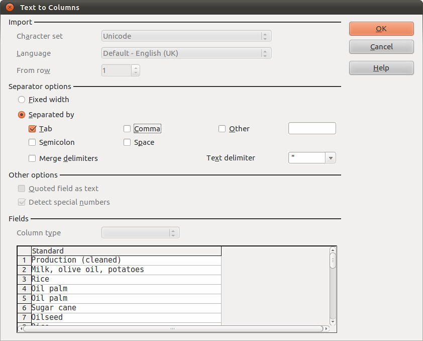
In “Separator options” area uncheck “tab” and check “comma”, as the items in our cells are separated by commas, and not tabs. In the “Fields” area you can see that for each comma the spreadsheet finds, it will move the data after that comma into a new column:
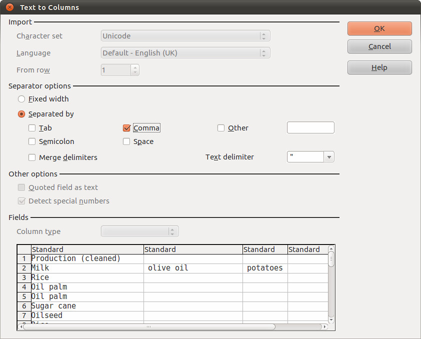
Select Okay, and watch what happens. Here’s how your data now looks:
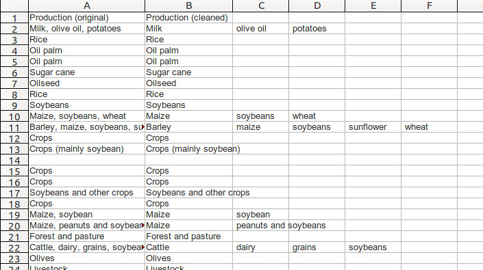
Do a few quick checks to see that nothing strange has happened. For example, check that the number of rows remains the same: there are 417 rows in the original data – this should not change. Also run your eye across a few of the rows to see things match.
Make one big list from the almighty mess
Why? This helps us find the unique items. There are over 700 individual items and many duplicates (to count them put =COUNTA(B2:P418) into a cell somewhere) and we can’t drill them down easily as they are currently structured. It’s easier if they are in a single column. To do this, we can use a little hack that occurs when you change file formats:
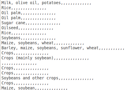
- Save your spreadsheet. Now delete column A and save it again with a new filename. Now save it again (yawn!), this time as a Text CSV.
Start up your favourite text editor (like Notepad on Windows, Gedit on Linux, or TextEdit on Mac) and open the Text CSV you just created. It’ll look something like this when it’s opened:
- Now copy and paste this text into a new document in Libre Office Writer. We will use Writer to process this data as text, before we return it to a spreadsheet for analysis. So, in Writer we will use the Find and Replace tool – it’s the same as in the spreadsheet – to create a single list:
- Replace all the commas with new lines: open the Find and Replace feature. Make sure “Regular Expressions” are enabled (look in “More Options”). In Find enter a single comma. In Replace enter n. This will replace every comma with a new line. There will now be lots of blank lines – don’t fret, this doesn’t matter.
- Select all the text (Ctrl-A) and copy it into the clipboard (Ctrl-C). Go back to your spreadsheet in Libre Office Calc. In a new worksheet select cell A1 and paste the text (Ctrl-V). The data will appear, but with lots of blank rows.
Select column A and go to Data → Pivot Table. Choose the options like this the below image.

- In a new worksheet a list of unique terms used to describe Production, arranged alphabetically, along with a count of how many times they occur, will appear:
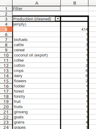
Remove duplicates and correct categories that are nearly the same
You can see immediately from the data above that there are many problems:
- “cofee” is mis-spelt, so is “forstry” (which should be ‘forestry’, which could be the same as ‘forest’)
- there are entries for “fruit” and “fruits”: which one is best?
This work is called ‘reconciliation’ and is a process designed to bring clarity to data. It involves looking through a list of terms and:
- identifying terms that mean the same thing and creating a new list
- applying the new list to the dataset.
We’ll go through these one by one.
Bring the data into a form in which it’s easy to do this task
- Copy the list of items from the Pivot Table you made above and add it into a new worksheet. Use CLEAN and TRIM on it, and then sort it alphabetically in ascending order.
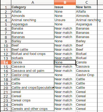
- Insert a row at the top. Label column A “Category”, Column B “Issue”, Column C “New Term”.
Identifying terms that mean the same thing
- Go down the list and look for terms that mean the same thing. Here are some things that should alert your suspicion about a term:
- Spelling mistakes e.g. “bananas” vs “banabas”
- Differences in case: “fruit” vs “Fruit”. Choose your case and stick to it.
- Multiples: “fruits” vs “fruit”. Choose which one you want to use. Adjectives: “sweet sorghum”, “winter barley”. If there’s a similar category, like just “barley”, it may make sense to remove this more specific category.
- Additional terms: “and” in the text eg. “Dairy and Grain farms”; “Citrus and Olives”; “Crops (sorghum)”. The rule is to have only one category in each cell. So delete one of the terms and add it to the list on its own if it doesn’t exist.
- Qualifying terms eg “beef cattle” vs “beef”. “Crops” vs “food crops”. Choose which one.
- In column B record what you think is the problem e.g. Near match, none, Spelling error. This will just help you keep track of the changes you make.
- When you’ve gone down the list and identified the problems, then make the changes in column C. Here’s what we did (we also ringed the suspected duplicates as we went along):
- Once you’ve done this, run Data → Pivot Table on your list of new terms (in Column C). You’ll see a huge difference.
- By removing duplicates, spelling and grammar differences and so on we have cut down the categories from 149 to 88, which is still quite an extensive list! Anyhow, we have a more useful controlled vocabulary. The next step is to apply this to the data, so it can help us with our analysis.
Edit the data to fit the more accurate list of categories
So in order to create a more accurate analysis of the GRAIN dataset we have narrowed down the categories used to describe the sorts of land use to which transacted land is put. The last step is to bring the data into compliance with these new terms. We can do this using a combination of three useful features of the spreadsheet:
- Conditional formatting: we mentioned this `above`_. It changes the formatting of a cell based on a rule that you give it eg. turn any cell in a given range red if it has the word “Sheep” in it. We can use this to highlight production categories that are not in our new improved list of categories.
- Data validation: this enables you to restrict what data is entered into a cell. So you specify a list of allowed values, and rather than type what you like into a cell you choose from a list. We can use this to make the changes to the data to bring it in line with the new categories, whilst reducing the risk of introducing more errors.
- Concatenation: this merges the contents of cells together. We will use it to put the improved data about production back together
The two things you will need are:
- the spreadsheet in which you used Text to Columns to separate out the terms used to describe land use
- your new, cleaned up list of terms taken from the previous pivot table.
Step 1: Find the items that need correcting
We can use the spreadsheet to find the items that need correcting by comparing the data we have to the new list of categories. Here’s how:
- In the worksheet where you have the data about production, make sure you have cleaned the data (using CLEAN and TRIM and paste special to remove the formulas).
- Have the split items in a worksheet called “Split”. Place your new list of categories in a worksheet called “Categories”. Select your list of categories. Go to Data → Define Range. This window will appear, which will enable us to make the list of categories into a “range” against which we can make comparisons:
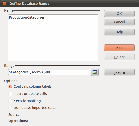
- You’ve already selected the list of categories, which you can see displayed in the Range area. Type ProductionCategories into the Name area and then select Add. We can now use this range.
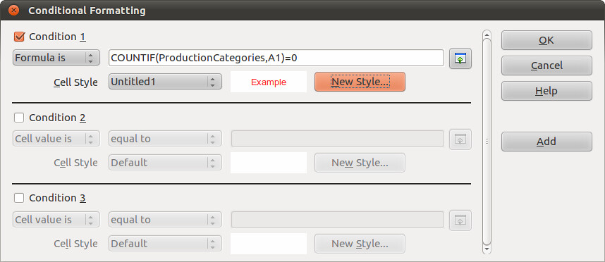
- Select all the data (Shortcut: Ctrl-A) in the worksheet called “Split”, where the data about production use is split across different columns. Go to Format → Conditional Formatting and make it look like the image below.
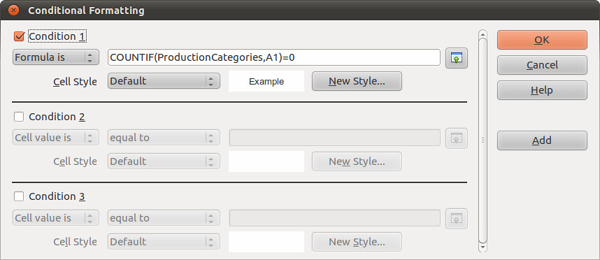
The formula to use is COUNTIF(ProductionCategories,A1)=0. Also, select “New Style”. A new window called “Cell Style” will pop up. In the “Font Effects” tab choose a colour and then select okay. We chose red, which is shown below:
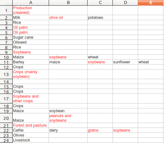
Select OK. This highlights in red the text in cells that are not found in the data range we have called “ProductionCategories”. The effect this has is to highlight the entries that we have to now correct. You spreadsheet will look like this:
Step 2: Correct these entries
Now we know where to look, we can make corrections to the data. The way to do this is to introduce data validation to the spreadsheet. This restricts the data that can be entered into a cell.
- Select the complete dataset in the worksheet called ‘Split”, where you’ve just highlighted the values that don’t appear on the improved list of categories. Go to Data → Validity.
- In the window that opens, make the fields look like those in the image below:
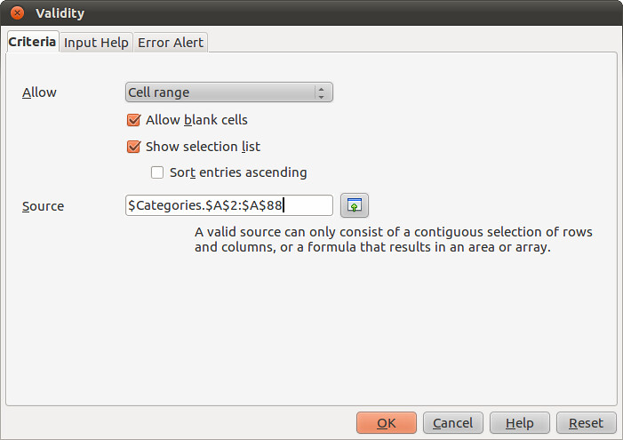
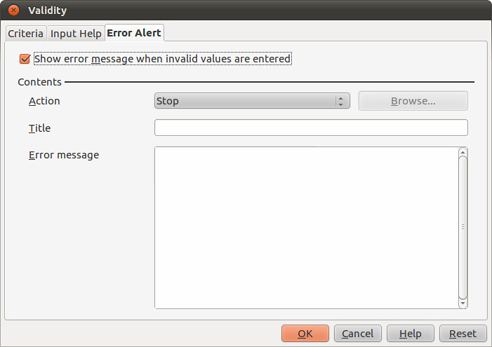
What this does is tell the spreadsheet that the only values that it should allow you to enter come from the list to be found in Cells A2:A88 of the worksheet called “Categories”. In others words: your list of categories. We also need to decide what to do when a value that isn’t on the list is entered. Select “Error Alert” and make it look like this to stop any non-list values being entered:
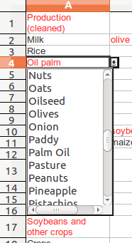
Click OK, and go to a cell with red text in it and click on it. You’ll see that a little drop down selector on the right hand side of the cell.
Click on it to display the list of ‘approved’ terms:
You can now go through the data, correcting it to remove the errors and make it more useful for analysis. There are a few things to watch out for:
- As you go through, increasingly you can use keyboard shortcuts and auto-complete and rely on the validation to tell you when you’ve typed a wrong entry.
- When you have changed a value, notice that the text changes to colour to show that it is now a recognised term. When there’s no more red, you’re done.
- With values like “Soyabean and other crops”, you should change it to “Soybean” and then add a new entry for “Crops”. Don’t forget!
Step 3: put it all back together again
We will take the improved data about land use and re-incorporate it into the full dataset.
- In you first worksheet, where you have been progressively cleaning the data, insert 15 columns to the right of Column F. Take the data from the worksheet that you validated the production category data in and copy it across into the new columns. If you didn’t put column heading, remember to paste starting in Row 2. You’ll be able to see the original data in Column F, and the separated about and cleaned data in Columns G to S.
- What we need to do now is put the clean data back into a single cell. We can do this with the CONCATENATE function. This allows you to take data from different cells and blend it into one. For example:
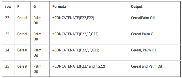
- We can blend data from other cells (which we called ‘referencing’), with other text to make it more readable. The examples above show how this works.
- Now let’s apply it to the data in our spreadsheet. In cell T2 insert the following formula:
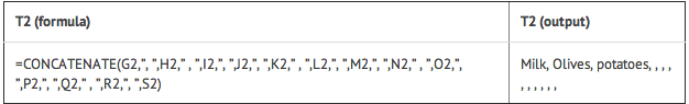
- It looks messy, but follow the logic. It looks across row 2 in columns G to S for data, and then prints it with a comma in between. We don’t know which cells have data in them precisely, so there is a list of trailing commas which print where a cell is empty. We can get rid of these easily with the LEFT and SEARCH formulas we used `above`_. In cell U2:
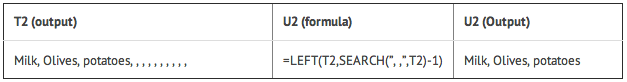
- So, with these two formulas in place, they can be copied down the spreadsheet to complete the operation. The only row that this doesn’t work for is row 94, Temasek’s purchase of land in China. You can correct it by hand :)
- The final step is to make the new data usable. If you’re confident the work is done, insert column to the left of the original column F called Production. Call this new Column G “Production (cleaned)”. Select all the data in Column T (rows 2 to 417), move the cursor and use Paste Special to insert it into Column G.
- You can now either delete or hide columns H to W in which you’ve been working.
Step 4: using the cleaned data about types of production land use
You can repeat the steps that we outlined in Problem 4 above, using the standard filters to build queries on the cleaned data in column G. This time you will not have problems with inconsistencies, mis-spellings and so on.
Finishing touches
- Columns A and C of the GRAIN data both record names of states. To check for errors here we copied the data from both columns into a single column, and created a pivot table that showed the list of unique values recorded in both columns. The only errors were a mis-spelling of Germany (“Gemany”) and the use of “West Africa”, which is a region not a state. We corrected both, including a note in the “Summary” cell if further clarity was needed.
- To complete this, apply the cleaning process outlined in Problem 5 above to Column D of the original GRAIN dataset, which records data about the sector. But for some issues with lower and upper case it does not share the same problem as the data about Production in column F. There are not obviously overlapping categories. To be certain, we ran CLEAN and TRIM again, and converted everything to sentence case (the formula is =PROPER(CLEAN(TRIM(cell reference))).
- In Column H (Status of Deal), we altered three entries that had additional text not in the categories Done, In Process, Proposed, Suspended, MOU signed. The information carried by this text was already continued in the Summary (column I).